Data Collection
To address our research objectives, we selected 100 lakes across Canada within the native range of Walleye (Fig.1). To ensure an even spread across provinces, 20 lakes were selected from each of Alberta, Saskatchewan, Manitoba, Ontario, and Québec. We used systematic random sampling when selecting sites to capture lakes at a range of latitudes and longitudes. We obtained mean lake depth (m) for each lake selected and generated two depth classes (shallow and deep) based on numerical values on either side of the median (5.02 m). Values above the median (> 5.02 m) were considered deep, while values below the median (< 5.02 m) were considered shallow. Where mean lake depth was unavailable, lake depth was inferred based on a linear area-depth relationship derived from lakes where both depth and area data were available. To obtain mean annual temperature (MAT) for each lake, we used the ClimateNA v5.10 software package, available at http://tinyurl.com/ClimateNA, based on methodology described by Wang et al. (2016). We also used this method to obtain a future climate scenario projection for the year 2085 under the RCP 8.5 warming scenario. We chose this particular warming scenario because it is the most dramatic, thus represents the ‘worst case scenario’. We believe displaying the ‘worst case scenario’ is an effective strategy to promote management action.
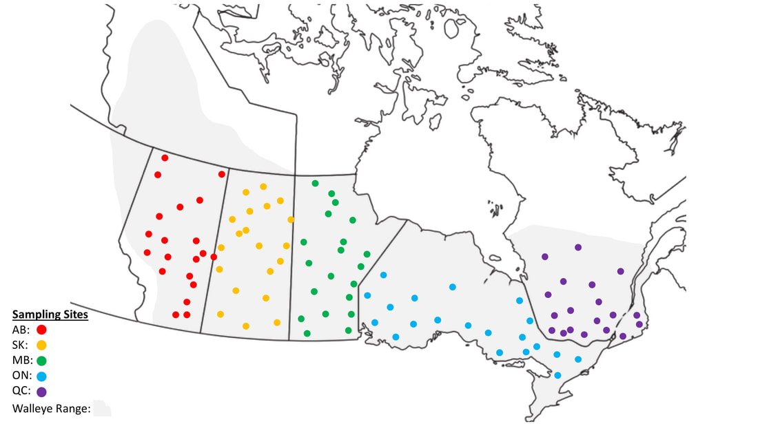
Figure 1. Map of the study area in Canada and lakes sampled in our study (n = 100).
To address our hypothesis that temperature influences walleye fitness, we reviewed literature on optimal walleye growing temperatures to create a parabolic equation representing the relationship between MAT and mean walleye total length (TL; mm) (Lester et al. 2004; Van Zuiden et al. 2016). Total length is used to assess overall population health and fish fitness (Önsoy et al. 2011; Fig. 2). We also derived linear and exponential equations to compare and contrast with the parabolic model. We used the Akaike Information Criterion (AIC) to compare the relative fit of each model on the relationship between MAT and TL (Burnham and Anderson 2002). We report AIC, ΔAIC, and AIC weight for each model.
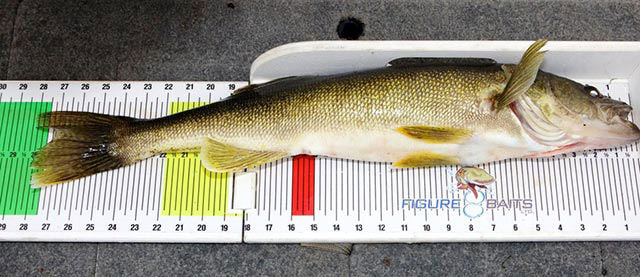
Figure 2. Photograph depicting the measurement of total length (mm) of a walleye (Sander vitreus). Source: https://anglers.travelmanitoba.com/master-angler-program/rules/.
To address our hypothesis that depth and angling pressure influence walleye abundance, we reviewed literature on the effects of angling pressure and lake depth on the relative abundance of fish species. Following recommendations from Maunder and Punt (2004) and Gulland (1969), we used catch per-unit effort (CPUE) as a measure of relative abundance. We created an ANCOVA to model the effect of lake depth, angling pressure, and lake area on the abundance of walleye in each lake (Bannerot and Austin 2011; Maunder and Punt 2004).
Statistical Analysis
1. Non-Linear Regression
Non-linear modelling is a suitable alternative to linear modelling when the shape of your response variable is not normal but you want to explore biologically meaningful relationships between continuous variables. In our case, TL assumed a shape similar to a parabolic or exponential function when plotted against our independent variable MAT. This relationship was expected as the growth curves of many fish exhibit parabolic responses to temperature in which there is a lower and upper limit to growth, as well as a thermal optimum (Bozek et al. 2011; Alofs et al. 2014; Hansen et al. 2017). While we could have employed data transformations in an attempt to force our response to a normal distribution, many transformations result in bias when back-transforming to enable interpretations of effect size. Alternatively, if we had multiple predictor variables we may have used a General Additive Model (GAM) which would have enabled the interpretation of non-linear data across the effects of multiple predictors. Ultimately, we opted to employ non-linear regression to simplify our analysis given biological considerations (the effect of temperature on optimal growth in walleye.
To determine the effect of MAT (°C) on TL (mm) we created three models: 1) parabolic (non-linear), 2) linear, and 3) exponential (non-linear). We fitted these models to our observed data. Non-linear regression analyses require one or more independent variables, and for the data to be well represented by the model. To avoid overfitting our models (and to test data representation), we used AIC (Burnham and Anderson 2002) to select the most supported model. According to Burnham and Anderson (2002), the model with the lowest AIC value is the most parsimonious, or the ‘best’. In other words, AIC balances model fit with model complexity. Models with ΔAIC < 2.00 were considered equally supported (Burnham and Anderson 2002).
2. Analysis of Covariance (ANCOVA)
An analysis of variance (ANOVA) tests the effects of 2 or more categorical variables on a continuous dependent variable. The results from an ANOVA test reveal if the means of two or more groups are significantly different from each other. An analysis of covariance (ANCOVA) functions in the same way as an ANOVA, with the ability to control for the effects of an additional continuous variable (covariate). In ecological research ANCOVAs allow for environmental variation to be included in the model. Like ANOVA, an ANCOVA assumes that the data is normally distributed, that there is homogeneity of variance, and that observations are independent. An additional assumption specific to ANCOVA is that the selected covariate is independent of treatment effects.
We modelled the effect of depth and angling pressure on CPUE using ANCOVA. CPUE was the continuous response variable, depth and angling pressure were both independent class variables, and lake area was a covariate (continuous). ANCOVA enabled us to test for significant differences in CPUE for each categorical variable. ANCOVA also allowed us to account for potential variation in CPUE caused by lake area. Our data meets the most important assumption of ANOVA, which is the independence of observations. Our data do not meet the assumptions of normality and homogeneity of variances, however due to the central limit theorem, these assumptions for ANOVA can be ignored. Specifically, P-values are calculated from sample means, which are always normally distributed for sample sizes greater than ~10. Alternative statistical tests included a simple ANOVA or pairwise t-tests, however these do not permit testing of interaction effects or covariates. Because we are interested in potential interactions between lake depth and angling pressure, as well as the effect of lake area, we chose to use ANCOVA.
